Effect of increasing water vapor improves match after 2001 at http://globalclimatedrivers2.blogspot.com
Cause of Global
Climate Change
Introduction
This monograph is a culmination of more than eight years of
work which has now quantified the contribution of atmospheric carbon dioxide
(CO2) change to average global temperature change and identified the
factors which explain average global surface temperature (AGT) change since
before 1900.
The word ‘trend’ is used here for temperatures in two
different contexts. To differentiate, α-trend applies to averaging-out the fluctuations
in reported average global temperature measurements to produce the average
global temperature oscillation resulting from the net of ocean surface temperature
oscillations. The term β-trend applies to the slower average energy change of
the planet which is associated with change to the average temperature of the
bulk volume of the material (mostly ocean water) involved.
The Model
Most modeling of global climate has been with Global Climate
Models (GCMs) where physical laws are applied to hundreds of thousands of
discreet blocks and the interactions between the discreet blocks are analyzed
using super computers with an end result being calculation of the AGT
trajectory. This might be described as a ‘bottom up’ approach. Although
theoretically promising, multiple issues currently exist with this approach,
some of which are discussed at [1]. Growing separation between calculated and
measured AGT as shown, e.g. at [2], discloses
that nearly all of the more than 100 current GCMs are obviously faulty. The few
which appear to follow measurements might even be statistical outliers of the
‘consensus’ method.
The approach in the analysis presented here is ‘top down’.
This type of approach has been called ‘emergent structures analysis’. As
described by Dr. Roy Spencer in his book The great global warming Blunder, “Rather
than model the system from the bottom up with many building blocks, one looks
at how the system as a whole behaves.” That approach is used here with strict
compliance with physical laws.
The basis for assessment of AGT is the first law of thermodynamics,
conservation of energy, applied to the entire planet as a single entity. Much
of the available data are forcings or proxies for forcings which must be
integrated (mathematically as in calculus, i.e. accumulated over tme) to
compute energy change. Energy change divided by effective thermal capacitance
is temperature change. Temperature change is expressed as anomalies which are
the differences between annual averages of measured temperatures and some
baseline reference temperature; usually the average over a previous multiple
year time period. (Monthly anomalies, which are not used here, are referenced
to previous average for the same month to account for seasonal norms.)
The model is expressed in this equation:
Tanom = (A,y)+thcap-1 * Σyi=1895
{B*[S(i)-Savg] + C*ln[CO2(i)/CO2(1895)] – F
* [(T(i)/T(1895))4 – 1]} + D (1)
Where,
Tanom =
Calculated average global temperature anomaly with respect to the baseline of
the anomaly for the measured temperature data set, K
A = highest-to-lowest
extent in the saw-tooth approximation of the net effect on planet AGT of all ocean
cycles, K
y = year
being calculated
(A,y) = value
of the net effect of ocean cycles on AGT in year y (α-trend), K
thcap =
effective thermal capacitance [3] of the
planet = 17±7 W yr m-2 K-1
1895 =
Selected beginning year of acceptably accurate world wide temperature
measurements.
B = combined
proxy factor and influence coefficient for energy change due to sunspot number
anomaly change, W yr m-2
S(i) =
average daily Brussels International sunspot number V1 [4] or V2 [5,6] in year
i
Savg =
average sunspot number = 34 (approximate average 1610-1940) for V1 and 62 for
V2
C = influence
coefficient for energy change due to CO2 change, W yr m-2
CO2(i) =
carbon dioxide level in year i, e.g. ppmv
CO2(1895) =
carbon dioxide level in 1895, same units as CO2(i) (Law Dome 294.8 ppmv)
F = 1 or 0 to
account for change to Stephan-Boltzmann radiation from earth due to AGT change
or not, W yr m-2
T(i) = AGT
calculated by adding 287.1 to the calculated anomaly, K
T(1895) = AGT
in 1895 = 286.74 K
D = offset
that shifts the calculated trajectory vertically on the graph, without changing
its shape, to best match the measured data, K
Accuracy of the model is determined using the Coefficient of
Determination, R 2, to compare calculated AGT with measured AGT.
Approximate effect on
the planet of the net of ocean surface temperature (SST)
The average ocean surface temperature oscillation is only
about ±1/6 K so it does not significantly
add or remove planet energy. The net influence of SST oscillation on
reported AGT is defined as α-trend. In the decades immediately prior to 1941
the amplitude range of the trends was not significantly influenced by change to
any candidate internal forcing effect; so the observed amplitude of the effect
on AGT of the net ocean surface temperature trend anomaly then, must be
approximately the same as the amplitude of the part of the AGT trend anomaly
due to ocean oscillations since then. This part is approximately 0.36 K total highest-to-lowest
extent with a period of approximately 64 years (verified below).
The AGT trajectory (Figure 8) suggests that the least-biased
simple wave form of the effective ocean surface temperature oscillation is
approximately saw-toothed. Approximation of the sea surface temperature anomaly
oscillation can be described as varying linearly from –A/2 K in 1909 to
approximately +A/2 K in 1941 and linearly back to the 1909 value in 1973. This
cycle repeats before and after with a period of 64 years.
Because the actual magnitude of the effect of ocean
oscillation in any year is needed, the expression to account for the
contribution of the ocean oscillation in each year to AGT is given by the
following:
ΔTosc = (A,y) K (degrees) (2)
where the contribution of the net of ocean oscillations to
AGT change is the magnitude of the effect on AGT of the surface temperature
anomaly trend of the oscillation in year y, and A is the maximum highest-to-lowest extent of the effect on AGT of
the net ocean surface temperature oscillation.
Equation (2) is graphed in Figure 1 for A=0.36.

Figure 1: Ocean surface
temperature oscillations (α-trend) do not significantly affect the bulk energy
of the planet.
Comparison of
approximation with ‘named’ ocean cycles
Named ocean cycles include, in the Pacific north of 20N,
Pacific Decadal Oscillation (PDO); in the equatorial Pacific, El Nino Southern
Oscillation (ENSO); and in the north Atlantic, Atlantic Multidecadal
Oscillation (AMO).
Ocean cycles are perceived to contribute to AGT in two ways:
The first is the direct measurement of sea surface temperature (SST). The
second is warmer SST increases atmospheric water vapor which acts as a forcing
and therefore has a time-integral effect on temperature. The approximation,
(A,y), accounts for both ways.
SST data is available for three named cycles: PDO index,
ENSO 3.4 index and AMO index. Successful accounting for oscillations is
achieved for PDO and ENSO when considering these as forcings (with appropriate
proxy factors) instead of direct measurements. As forcings, their influence
accumulates with time. The proxy factors must be determined separately for each
forcing. The measurements are available since 1900 for PDO [7] and ENSO3.4 [8].
This PDO data set has the PDO temperature measurements reduced by the average
SST measurements for the planet.
The contribution of PDO and ENSO3.4 to AGT is calculated by:
PDO_NINO = Σyi=1900 (0.017*PDO(i) +
0.009 * ENSO34(i)) (3)
Where:
PDO(i) =
PDO index [7] in year i
ENSO34(i) =
ENSO 3.4 index [8] in year i
How this calculation compares to the idealized approximation
used in Equation (2) with A = 0.36 is shown in Figure 2.

Figure 2: Comparison
of idealized approximation of ocean cycle effect and the calculated effect from
PDO and ENSO.
The AMO index [9] is formed from area-weighted and de-trended
SST data. It is shown with two different amounts of smoothing in Figure 3 along
with the saw-tooth approximation for the entire planet per Equation (2) with A
= 0.36.

Figure 3: Comparison
of idealized approximation of ocean cycle effect and the AMO index.
The high coefficients of determination in Table 1 and the
comparisons in Figures 2 and 3 corroborate the assumption that the saw-tooth
profile with a period of 64 years provides adequate approximation of the net
effect of all named and unnamed ocean cycles in the calculated AGT anomalies.
Atmospheric carbon
dioxide
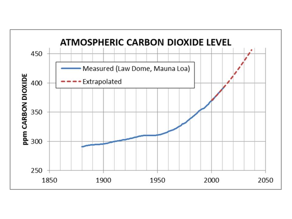
The level of atmospheric carbon dioxide (CO2) has
been widely measured over the years. Values from ancient times were determined
by measurements on gas bubbles which had been trapped in ice cores extracted
from Antarctic glaciers [10]. Spatial variations between sources have been
found to be inconsequential [19]. The best current source for atmospheric
carbon dioxide level [11] is Mauna Loa, Hawaii. Extrapolation to future CO2
levels, shown in Figure 4, is accomplished using a second-order curve fit to
data measured at Mauna Loa from 1980 to 2012.
EPA mistake

At
https://www3.epa.gov/climatechange/ghgemissions/gwps.html the EPA asserts Global Warming Potential
(GWP) is a measure of “effects on the Earth's warming” with “Two key ways in
which these [ghg] gases differ from each other are their ability to absorb
energy (their "radiative efficiency"), and how long they stay in the
atmosphere (also known as their "lifetime").”
The EPA calculation
overlooks the very real phenomenon of THERMALIZATION. When a ghg molecule absorbs a photon it immediately (within about
0.0002 microsecond at sea level conditions) bumps in to other molecules. If
this happens before the molecule emits a photon, part of the molecule’s energy
is transferred to the other molecule(s) greatly reducing the probability a
photon will be emitted. The process of photon absorption and transfer of energy
is called thermalization. The transfer of energy is gas-phase thermal
conduction and explains most of how the atmosphere, which is about 98% non-ghg
gases, is warmed. A common observation of thermalization by way of water vapor
is cloudless nights cool faster when absolute water vapor content is lower.
The only way that
energy can significantly leave earth is by thermal radiation. Only solid or
liquid bodies and ghg can radiate/emit in the wavelength range of terrestrial
radiation. Non-ghg gases must transfer energy to ghg gases (or liquid or solid
bodies) for the energy to be radiated. The non-ghg to ghg energy transfer with
subsequent radiation is called reverse thermalization. The spike observed in
top-of-atmosphere scans at the nominal absorption/emission wavelength of
non-condensing ghg molecules results from reverse-thermalization.
There are about 35
times as many water vapor molecules as CO2 molecules in the troposphere and
each water vapor molecule can absorb/emit energy at hundreds of wavelengths
compared to only one (broadened to a range of about 14-16 microns at sea level)
for CO2. Thus, in the troposphere, reverse-thermalization is thousands of times
more likely to be to a water vapor molecule than to a CO2 molecule. The same
holds for all non-condensing ghg.
Therefore, because
absorbed terrestrial radiation by noncondensing ghg becomes thermalized, GWP,
as calculated by the EPA, is not a measure of their relative influence on
average global temperature. As a consequence non-condensing ghgs are
insignificant compared to water vapor in influencing average global
temperature.
Figure 5 provides insight as to the fraction of atmospheric CO2 for various times and conditions. The planet came perilously close to extinction of all plants and animals due to the low level of CO2 at the end of the last glaciation. For plant growth, at the current level the atmosphere is impoverished for CO2.
Figure 5 provides insight as to the fraction of atmospheric CO2 for various times and conditions. The planet came perilously close to extinction of all plants and animals due to the low level of CO2 at the end of the last glaciation. For plant growth, at the current level the atmosphere is impoverished for CO2.

Figure 5: Typical
values for CO2 levels.
Sunspot numbers
Sunspots have been regularly recorded since 1610, The most
widely accepted data set is the average daily Brussels International sunspot
numbers. They compensate for increased instrument sensitivity over the years to
put all values on a common basis. This set is shown in Figure 6.

Figure 6: Brussels
International sunspot numbers. (V1) [4]
Sunspot numbers (SSN) are seen to be in cycles each lasting
approximately 11 years. The current cycle, called 24, has been comparatively
low, has peaked, and is now in decline.
The Maunder Minimum (1645-1715), an era of extremely low SSN,
was associated with the Little Ice Age. The Dalton Minimum (1790-1820) was a
period of low SSN and low temperatures. An unnamed period of low SSN (1880-1930)
was also accompanied by comparatively low temperatures.
An assessment of this is that sunspots are somehow related
to the net energy retained by the planet, as indicated by changes to average
global temperature. Fewer sunspots are associated with cooling, and more
sunspots are associated with warming. Thus the hypothesis is made that SSN are
proxies for the rate at which the planet accumulates (or loses) radiant energy
over time. Therefore the time-integral of the SSN anomalies is a proxy for the
amount of energy retained by the planet above or below breakeven.
Also, a lower solar cycle over a longer period might result
in the same increase in energy retained by the planet as a higher solar cycle
over a shorter period. Both magnitude and time are accounted for by taking the
time-integral of the SSN anomalies, which is simply the sum of annual mean SSN (each
minus Savg) over the period of study.
SSN change correlates with change to Total Solar Irradiance
(TSI). However, TSI change can only account for less than 10% of the AGT change
on earth. Because AGT change has been found to correlate with SSN change, the
SSN change must act as a catalyst on some other factor (perhaps clouds) which
have a profound effect on AGT.
In 2015 historical (V1) SSN were reevaluated in light of
current perceptions and more sensitive instruments. Although there are
substantial yearly differences, version 2 (V2) SSN, on average, tend to be
about 20% higher than V1.
Application of Equation 1 using the same method as before
results in slightly different influence coefficients and a substantially
different value for Savg. However, the end result of influence of CO2
on AGT is not markedly different. V2 SSN are shown in Figure 7.
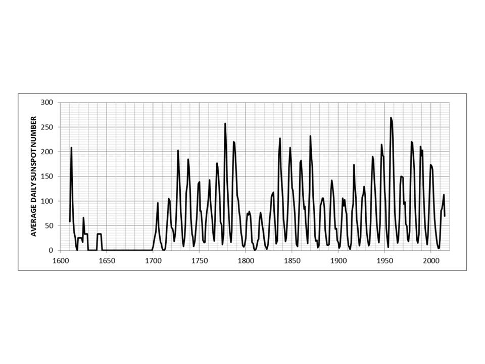
Figure 7: V2 SSN [5]
The highest Coefficient of Determination (R2 ) over
the period 1895-2015 for V1 was found with Savg = 34. For V2 SSN Savg = 62.
The values for Savg are subject to two constraints.
Initially they are determined as that which results in derived coefficients and
maximum R2. However, calculated values must also result in rational
values for calculated AGT at the depths of the Little Ice Age. The necessity to
calculate a rational LIA AGT is a somewhat more sensitive constraint. The
selected values for Savg result in calculated LIA AGT of approximately 1 K less
than the recent trend which appears rational and is consistent with most LIA
AGT assessments.
AGT measurement data
sets
In earlier work, in an attempt to avoid bias, reported data
were ‘normalized’ to HadCRUT4 data through 2012 as described at [12]. Reported
data were essentially unchanged by the reporting agencies prior to 2012. Since
then temperature data, especially land temperature data, have been changed
which detracts from their applicability in any correlation.
All data sources appear to be fairly similar. Rapid
year-to-year changes in reported temperature anomalies are not physically
possible for true energy change of the planet. The sharp peak in 2015, which
coincides with an especially extreme El Nino, is especially distorting. It, at
least in part, will be compensated for by an equally extreme La Nina which is
sure to follow. In each data set the El Nino spike is compensated for by
replacing reported AGT for 2013-2015 with the average 2002-2012.
A further bit of
confusion is introduced by satellite determinations. Anomalies they report as
AGT anomalies are actually for the lower troposphere (LT), have a different
reference temperature (reported anomalies determined using satellite data are
about 0.2 K lower), and appear to be somewhat more volatile (about 0.15 K
further extremes than surface measurements) to changes in forcing.
At this point, it appears reasonable to consider two
temperature anomaly data sets extending through 2015:
1) The set used
previously [12] through 2012 with extension 2013-2015 set at the average
2002-2012 (when the trend was flat) at 0.4864 K above the reference temperature.
2) Current
(5/27/16) HadCRUT4 data set [13] through 2012 with 2013-2015 set at the average
2002-2012 at 0.4863 K above the reference temperature.
These are co-plotted on Figure 8.

Figure 8: Examples of
AGT anomaly data
The sunspot number
anomaly time-integral is a proxy for a primary driver of the temperature
anomaly β-trend
By definition, energy change divided by effective thermal
capacitance is temperature change.
In all cases in this document, coefficients (A, B, C, D
& F) which achieved maximum R2 for unsmoothed data sets were not
changed when calculating R2 for smoothed data.
Incremental convergence to maximum R2 is
accomplished by sequentially and repeatedly adjusting the coefficients. The
process is analogous to tediously feeling the way along a very long and narrow
mathematical tunnel in 4-dimensional mathematical space. The ‘mathematical
tunnel’ is long and narrow because the influence on AGT determined by the SSN
anomaly time-integral, at least until the last decade or so, is quite similar
to the influence on AGT as determined by the rise in atmospheric CO2
level.
Measured temperature anomalies in Figure 9 use Data Set 1
shown in Figure 8. The excellent match of the up and down trends since before 1900 of
calculated and measured temperature anomalies, shown here in Figure 9, and, for
5-year moving average smoothed temperature anomaly measurements, in Figure 10, demonstrate
the usefulness and validity of the calculations. All reported values since
before 1900 are within the range ±2.5 sigma (±0.225 K) from the calculated
trend. Note: The variation is not in the method, or the measuring instruments
themselves, but results from the effectively roiling (at this tiny magnitude of
temperature change) of the object of the measurements.
Projections until 2020 use the expected sunspot number trend for
the remainder of solar cycle 24 as provided [6] by NASA. After 2020 the ‘limiting
cases’ are either assuming sunspots like from 1924 to 1940 or for the case of
no sunspots which is similar to the Maunder Minimum.
Some noteworthy volcanoes and the year they occurred are also
shown on Figure 9. No consistent AGT response is observed to be associated with
these. Any global temperature perturbation that might have been caused by
volcanoes of this size is lost in the natural fluctuation of measured temperatures.
Much larger volcanoes can cause significant temporary global cooling
from the added reflectivity of aerosols and airborne particulates. The Tambora
eruption, which started on April 10, 1815 and continued to erupt for at least 6
months, was approximately ten times the magnitude of the next largest in
recorded history and led to 1816 which has been referred to as ‘the year
without a summer’. The cooling effect of that volcano exacerbated the already
cool temperatures associated with the Dalton Minimum.

Figure 9: Measured
average global temperature anomalies with calculated prior and future trends
(Data Set 1) using 34 as the average daily sunspot number and with V1 SSN. R
2 = 0.913463

Figure 10: Same as
Figure 9 but with 5-year running average of measured temperatures. R2
= 0.978887. Data Set 1, V1 SSN.
Coefficients in Equation (1) which were determined by
maximizing R2 identify maximums for each of the factors explicitly
considered. Factors not explicitly considered (such as unaccounted for residual (apparently random) variation in reported
annual measured temperature anomalies, aerosols, CO2, other
non-condensing ghg, volcanoes, ice change, etc.) must find room in the
unexplained residual, and/or by occupying a fraction of the effect occupied by
each of the factors explicitly considered. The derived coefficients and other
results are summarized in Table 1. Note that a coefficient of determination, R2
= 0.978887 means a near-perfect correlation coefficient of 0.9894.
The influence of the net effect of factors other than the
net effect of ocean cycles on AGT can be calculated by excluding the α-trend
from the AGT which was calculated using Equation (1). For the values used in
Figure 9, this results in the β-trend as shown in Figure 11. Note that in 2005
the anomaly from other than α-trend, as shown in Figure 11, is A/2 lower than
the calculated trend in Figures 9 and & 10 as it should be.

Figure 11: Anomaly
trend (β-trend). Equation (1) except summation starts at i = 1610 and excluding
α-trend. Data Set 1, V1 SSN.
How the β-trend could
take place
Although the
connection between AGT and the sunspot number anomaly time-integral is
demonstrated, the mechanism by which this takes place remains somewhat speculative.
Various papers have been written
that indicate how the solar magnetic field associated with sunspots can
influence climate on earth. These papers posit that decreased sunspots are
associated with decreased solar magnetic field which decreases the deflection
of and therefore increases the flow of galactic cosmic rays on earth.
Henrik Svensmark, a Danish physicist, found that increased
flow of galactic cosmic rays on earth caused increased low altitude (<3 km)
clouds and planet cooling. An abstract of his 2000 paper is at [14]. Marsden
and Lingenfelter also report this in the summary of their 2003 paper [15] where
they make the statement “…solar activity increases…providing more shielding…less low-level cloud cover… increase surface air
temperature.” These findings have been further corroborated by the cloud
nucleation experiments [16] at CERN.
These papers [14,15] associated the increased low-altitude clouds with
increased albedo leading to lower temperatures. Increased low altitude clouds
would also result in lower average cloud altitude and therefore higher average
cloud temperature. Although clouds are commonly acknowledged to increase
albedo, they also radiate energy to space so increasing their temperature
increases S-B radiation to space which would cause the planet to cool.
Increased albedo reduces the energy received by the planet and increased
radiation to space reduces the energy of the planet. Thus the two effects work
together to change the AGT of the planet.
Simple analyses [17] indicate that either an increase of approximately 186
meters in average cloud altitude or a decrease of average albedo from 0.3 to
the very slightly reduced value of 0.2928 would account for all of the 20th
century increase in AGT of 0.74 K. Because the cloud effects work together and
part of the temperature change is due to ocean oscillation (low in 1901, 0.2114
higher in 2000), substantially less cloud change would suffice.
Hind Cast Estimate
Average global temperatures were not directly measured in
1610 (thermometers had not been invented yet). Recent estimates, using proxies,
are few. The temperature anomaly trend that Equation (1) calculates for that
time is roughly consistent with other estimates. The decline in the trace
1615-1700 on Figure 11 results from the low sunspot numbers for that period as
shown on Figure 6.
As a possibility, the period and amplitude of oscillations
attributed to ocean cycles demonstrated to be valid after 1895 are assumed to
maintain back to 1610. Equation (1) is modified to begin integration in 1610. The
coefficient D is changed to make the calculated temperature in 2005 equal to
what it is in Figure 9.
Temperature anomalies thus calculated, estimate possible
trends since 1610 and actual trends of reported temperatures since they have
been accurately measured world wide.
This assessment is shown in Figure 12.

A survey [18] of non-tree-ring global temperature estimates
was conducted by Loehle including some for a period after 1610. Simplifications
of the 95% limits found by Loehle are also shown on Figure 12. The spread
between the upper and lower 95% limits are fixed, but, since the anomaly
reference temperatures might be different, the limits are adjusted vertically
to approximately bracket the values calculated using the equations. The fit
appears reasonable considering the uncertainty of all values.
Calculated temperature anomalies look reasonable back to 1700 but indicate
higher temperatures prior to that than most proxy estimates. They are, however,
consistent with the low sunspot numbers in that period. They qualitatively
agree with Vostok, Antarctica ice core data but decidedly differ from Sargasso Sea
estimates during that time (see the graph for the last 1000 years in Reference 19).
Worldwide assessments of average global temperature, that far back, are sparse
and speculative. Ocean oscillations might also have been different from
assumed.
Data Set 2 with V2
SSN
Similarly, graphs 13,14 and 15 were determined for Data Set
2 and V2 SSN using Equation (1).


Figure 14: β-trend,
HadCRUT4 (as of 5/28/16) 2012 and earlier, 2013-2015 flat at 0.4863 K. V2 SSN.

Projection from 1990
Figure 16 shows the calculation using Equation (1) with
coefficients determined using HadCRUT4 measured temperatures to 1990. The
calculated temperature trend in 2020 with the 1990 projection is 0.08 K cooler
than the projection using Data set 2 which is through 2015.

Figure 16: Same as
Figure 13 except coefficients determined using data through 1990.
Imposed constraint of
limiting influence of CO2.
Figure 17 shows the AGT trajectory that occurs for the
condition that the CO2 level is arbitrarily constrained to the noted
limit. Same Equation (1), Data Set 2, V2 SSN as for Figure 13.

Figure 17: Calculated
trajectory if influence of CO2 is constrained. Data Set 2.
Step changes in AGT
Interpretation of a reported sudden AGT increase (or
decrease) as planet energy increase (or decrease) is physically impossible
because of the huge effective thermal capacitance which results in a 5-year
time constant [3] for thermal response of the planet to a step change in
forcing.
Influence of
atmospheric CO2 on AGT
The temperature increase through 2015 attributable to CO2
is the net of the increase from CO2 and the decrease from added S-B
radiation due to the part of the temperature rise above the 1895 value of
286.74 K attributable to CO2. The net effect is designated ΔTCO2.
At least until the last decade or so, the influence on AGT
due to CO2 has been quite similar to the influence on AGT determined
by the SSN anomaly time-integral. This similarity has resulted in calculation
of CO2 influence erroneously much greater than indicated by other
evidence. For example, in the late Ordovician Period the planet plunged into
and warmed up from the Andean/Saharan ice age all while the CO2
level was approximately ten times the present [20].
Values for the coefficients and results are summarized in
Table 1.
Table 1: A, B, C, D, F
refer to coefficients in Equation 1. The column headed # is a code identifying
the particular EXCEL file used.
#
|
Fig
|
Savg
|
OCEAN
A
|
SUN
B
|
CO2
C
|
Δ
D
|
F
|
R2
|
5-YR
R2
|
1895-2015
ΔTCO2 K
|
% CAUSE OF 1909-2005 AGT
CHANGE
|
|||
Sun
|
SEA
|
CO2
|
||||||||||||
T
|
9
|
34
|
.3285
|
.002727
|
.333
|
-.4365
|
1
|
.913463
|
.978887
|
.228
|
46.7
|
34.7
|
18.6
|
|
S
|
13
|
62
|
.3561
|
.002055
|
.427
|
-.4187
|
1
|
.904156
|
.981334
|
.291
|
38.3
|
37.8
|
23.9
|
|
Z
|
16
|
62
|
.3815
|
.002657
|
.198
|
-.4275
|
1
|
.901712
|
.978334
|
.135
|
49.2
|
39.9
|
10.9
|
|
X
|
17
|
62
|
.3975
|
.002910
|
.08
|
-.4325
|
1
|
.898797
|
.975017
|
.054
|
54.0
|
41.6
|
4.4
|
|
Note that the R2 decreases only about a half per
cent when the influence of CO2 on AGT is artificially constrained to
4.4% compared to the case (#S) for maximum R2.
Possible explanation of why CO2 change
has no significant effect on climate.
1) Firmly acknowledge the established fact
that gas molecules can absorb/emit photons only at specific discreet
wavelengths (which might be broadened from pressure, etc.). This fact makes
spectroscopy possible. Full spectrum (Plank’s law) Stephan-Boltzmann (S-B)
radiation applies to liquids and solids, not to gases.
2) From gas kinetics, the time between
atmospheric molecule collisions is extremely short (The Hyperphysics calculator
calculates approximately 0.0002 microsecond at sea level pressure and
temperature).
3) The elapsed time between absorption and
emission of a photon by a CO2 gas molecule is perhaps shorter at
higher temperature but must be greater than zero or there would be no evidence
that absorption-emission had occurred.
4) At sea level conditions, some or all of
the photon energy that is absorbed by a (so called) greenhouse gas (ghg)
molecule might be immediately transferred to other molecules by collision. The
process of absorbing a photon and transferring (thermal conduction in the gas)
the added energy to other molecules is called thermalization. A common
observation of thermalization by way of water vapor is that cloudless nights
cool faster when absolute water vapor content is lower.
5) The reduced radiation flux on both
sides of the 15 micron CO2 absorption line, as observed in most Top of
Atmosphere (TOA) measurements results because some of the EMR
energy absorbed by CO2 has been thermalized.
6) Terrestrial radiation is nearly all in
the wavelength range 6-100 microns. Thermalized energy carries no identity of
the molecule that absorbed it.
7) Jostling between the molecules
sometimes causes reverse-thermalization. At low to medium altitudes, EMR
emission stimulated by reverse-thermalization is mostly by way of water vapor. The
TOA spike at 15 microns results from reverse-thermalization to CO2 molecules
at very high altitude.
8) The thermalized radiation warms the
air, reducing its density, causing updrafts which are exploited by soaring
birds, sailplanes, and occasionally hail. Updrafts are matched by downdrafts
elsewhere, usually spread out but sometimes recognized by pilots and passengers
as ‘air pockets’ and micro bursts.
9) The population gradient of ghg
molecules, (especially water vapor above about 3 km, declining with increasing
altitude) favors radiation to space. Ghg molecules that emit a photon are
‘recharged’ by reverse-thermalization (or by absorbing a photon of appropriate
wave length).
10) Clouds (average emissivity about 0.5)
consist of solid and/or liquid water particles (each particle containing
millions of molecules) that radiate according to S-B law. Low and declining
amount of water vapor above clouds and widening molecule spacing allows increased
radiation directly to space with increased altitude.
11) The tiny increase in ghg from
increased CO2 causes absorption/thermalization to occur at slightly
lower altitude which very slightly increases the convection rate.
12) The increase in absorbing molecules
near the surface is at least partially compensated for by an equal percent increase
in emitting molecules high in the atmosphere radiating energy from the planet.
Because CO2
is only a trace gas in the atmosphere (approx. 0.04%), if CO2 change
does not cause significant temperature change, it cannot cause significant climate
change. Thus the CO2
change from burning fossil fuels has no significant effect on climate and
climate sensitivity (the effect on AGT of doubling CO2) is not
significant. Estimated magnitude is
Climate Sensitivity = 0.291 *
ln(2)/ln(400.31/294.8) = 0.66 K
The finding that
CO2 has no significant effect on climate might appear to conflict
with the known absorption of 15 micron radiation by CO2. Suspected
explanations for this include that there are so many more 'opportunities' for
absorption by water vapor molecules (hundreds of absorption lines per molecule
times number of molecules) that the added CO2 'opportunities' have
an insignificant effect (single absorption line in the range of significant
terrestrial radiation) and/or added TOA CO2 molecules emitting to
space compensate, at least in part, for the added molecules absorbing at low
altitude.
The EPA erroneously asserts global warming potential (GWP)
is a measure of “effects on the Earth's warming” with “Two key ways in which
these [ghg] gases differ from each other are their ability to absorb energy
(their "radiative efficiency"), and how long they stay in the
atmosphere (also known as their "lifetime").” [21].
The EPA calculation erroneously overlooks the fact that any effect the ghg
might have on temperature is also integrated over the “lifetime” of the gas in
the atmosphere so the duration in the atmosphere cancels out. Therefore GWP is
not a measure of the relative influence on average global temperature of ghgs
on a molecule basis.
Conclusions
Two factors can explain most of AGT change since before 1900.
They are ocean cycles, accounted for with an approximation, and, influence
quantified by a proxy; the SSN anomaly time-integral.
Others have looked at only amplitude or only duration
factors for solar cycles and got poor correlations with average global
temperature. The excellent correlation comes by combining the two, which is
what the time-integral of sunspot number anomalies does. Prediction of future
sunspot numbers more than a decade or so into the future has not yet been
confidently done.
As displayed in Figures 11 and 14, the β-trend shows the estimated true
average global temperature trend (the net average global energy trend) during
the planet warm up from the depths of the Little Ice Age.
The net effect of ocean oscillations is to cause the surface
temperature α-trend to oscillate above and below the β-trend. Equation (1)
accounts for both trends.
Figures 10 and 13 show the near perfect match with
calculated temperatures which occurs when random fluctuation in reported
measured temperatures is smoothed out with 5-year moving average.
Long term prediction of average global temperatures depends
primarily on long term prediction of sunspot numbers.
References:
1. Consensus
mistakes http://consensusmistakes.blogspot.com
2. Epic fail
of ‘consensus’ method http://www.drroyspencer.com/2013/06/still-epic-fail-73-climate-models-vs-measurements-running-5-year-means
3. Effective
thermal capacitance & time constant: Schwartz, Stephen E., (2007) Heat
capacity, time constant, and sensitivity of earth’s climate system, J. Geophys. Res., vol. 113, Issue D15102,
doi:10.1029/2007JD009373
4. V1
1700-2009 by year http://www.inference.phy.cam.ac.uk/sustainable/book/tex/GISS/spots.txt
V1 by month
thru April 2015 http://solarscience.msfc.nasa.gov/greenwch/spot_num.txt
5. V2 sunspot
numbers http://www.sidc.be/silso/datafiles
6. Graphic of
V2 Solar cycle 24: http://solarscience.msfc.nasa.gov/predict.shtml
7. PDO index http://jisao.washington.edu/pdo/PDO.latest
8. El Nino
3.4 index http://www.esrl.noaa.gov/psd/gcos_wgsp/Timeseries/Data/nino34.long.data
(Linked from http://www.cgd.ucar.edu/cas/catalog/climind/TNI_N34
)
10. CO2 level
at Law Dome, Antarctica: http://cdiac.ornl.gov/ftp/trends/co2/lawdome.combined.dat
11. Mauna Loa
CO2: ftp://aftp.cmdl.noaa.gov/products/trends/co2/co2_annmean_mlo.txt
12. Previous
measured AGT data set http://globaltem.blogspot.com
13. Current
HadCRUT4 data set: http://www.metoffice.gov.uk/hadobs/hadcrut4/data/current/time_series/HadCRUT.4.4.0.0.annual_ns_avg.txt
14. Svensmark
paper: Phys. Rev. Lett. 85, 5004–5007
(2000) http://prl.aps.org/abstract/PRL/v85/i23/p5004_1
15. Marsden
& Lingenfelter 2003, Journal of the
Atmospheric Sciences 60: 626-636 http://www.co2science.org/articles/V6/N16/C1.php
16. CLOUD experiment at CERN http://indico.cern.ch/event/197799/session/9/contribution/42/material/slides/0.pdf
17.
Sensitivity of AGT to clouds http://lowaltitudeclouds.blogspot.com
18. Loehle
non-tree-ring AGT http://www.econ.ohio-state.edu/jhm/AGW/Loehle/Loehle_McC_E&E_2008.pdf
19. 2008
assessment of non-condensing ghg http://www.middlebury.net/op-ed/pangburn.html
20.
Phanerozoic AGT & CO2: http://www.geocraft.com/WVFossils/Carboniferous_climate.html
21. EPA
determination of global warming potential of ghg: https://www3.epa.gov/climatechange/ghgemissions/gwps.html
Very interesting Dan. Do you offer an explanation for the
ReplyDeleteapparently wide divergence in "measured" temperatures vs.
modeled temperatures after 2010? (fig. 6 and 7). Thanks.
At least 3 factors contribute:
ReplyDelete1. Agencies reporting surface measurements have been changing the numbers to corroborate a global warming agenda.
2. The on-going super El Nino (very much like 1997-8, the effects of which were essentially cancelled out by the 1999 La Nina).
3. The way EXCEL does smoothing combined with what I assumed for decline rate from the El Nino (-0.013 K/yr which is OK for the long term trend but way too slow for coming down from an El Nino peak.)
Some of this is shown graphically at http://endofgw.blogspot.com
Hi Dan,
ReplyDeleteThis comment is not directly about this article. Your contact by email does not work for me. I just learned about you because of your comment on Roy Spencer's site about William Gray. I have quickly scanned some of your articles and the 5/12/2013 article Global Warming Made Simple (low level clouds) is specifically the one I want to discuss.
During this scanning I find you are a proponent of observation. I recently came up with a novel definition of science. Novel because I have never read it being written or heard it being spoken. Science is a method of learning solely based upon observation.
You clearly have skills that I do not but I believe I have a knowledge of observations that you may have not yet discovered in your scholarship. This because I, a chemist, have studied the greenhouse effect and other atmospheric phenomena for 40+ years.
I much prefer a private discussion than the public one like this. My email is jerry.semivision@gmail.com. So, hopefully you will respond by email.
Have a good day, Jerry L. Krause
Ph.D. physical chemistry, Oregon State University, 1969
Reblogged excerpts of this paper:
ReplyDeletehttps://rclutz.wordpress.com/2016/06/22/quantifying-natural-climate-change/
Hi Dan,
ReplyDeleteIt seems obvious that I have entered a phase of life where my memory sometimes fails me. For I had no memory of my comment of 4/22/2016. I come to your website from your recent comments at PSI because I liked what you wrote and I did not want to make any comment there. This because I am trying to keep my comments on the right column there as long as possible.
Having begun to read your 2/22/2016 monograph, I must admit that I did not read far. The reason for this is I have become convinced that a consideration of averaged anything is a waste of time. For average anything is not actually real anything. Better to compare the actual weather of a day with the actual weather of the next day. If the two weathers seem the same, try to answer the question: Why, of how, are they the same? If the two weathers appear to be different try to answer the questions: First, how are they different? Second, what factors seem to make them different?
And, maybe one could be lucky to encounter the weather of a day which is referred to as somethings occurring at Melbourne, Australia. For in information for tourists I read that sometimes in a single day the ‘normal’ weather of its four seasons can be experienced.
Newton is said to have stated: “If I have seen further than others, it is by standing on the shoulders of giants.” As you study climate, on whose shoulders do you stand? Because I know that climate is merely the average of observed weather that has been observed on a given day for many years, I consider we must study weather to begin to understand climate.
My giant is R. C. Sutcliffe and his 1966 book Weather and Climate. On page 33 of Chapter 4, The Classification of Clouds, he wrote: “Clouds which do not give rain, which never even threaten to give rain but which dissolve again into vapour before the precipitation stage is ever reached, have a profound effect on our climate.” I ask you: Where else can you find this statement so bluntly stated? Or, who do you know that has actually challenged this idea? From my reading most, not all, ignore clouds as a fundamental factor of anything except precipitation. Sure, clouds are generally considered to cool the temperature but I can cite observations that show clouds can increase the downwelling solar radiation reaching the earth’s surface. Which, even though they slightly reduce the downwelling solar radiation reaching the earth’s surface, can increase the observed maximum diurnal air temperatures observed over a sequence of consecutive days of these specific clouds. Curious?
What is your opinion of this article:
ReplyDeleteWash. Post: Scientists Detected a Major Change to Oceans Due to Warming Climate
JB - That refers to a Letter published in the Journal Nature. Letters have even less credibility than peer reviewed papers and about half of those are found to be wrong. The work used ocean models. Models often are biased to show the intended finding of researchers. The work is described as 'research synthesis'. The reported finding was a reduction of less than 2% in 60 years which they call a "major change". They also report that only 15% of this 2% is due to ocean warming.
ReplyDeleteThe oxygen content of the ocean is provided by plants in the ocean and removed by animals (fish, clams, etc.) and decaying stuff that was once living. It varies throughout the oceans depending on what is prevailing locally. IMO this reported 2% change in half a century, is not very meaningful and certainly no cause for alarm. The decline in solubility of oxygen with rising water temperature is a result of lab tests and has been known for at least a century.
Average global temperature (AGT) depends mostly on ocean temperature. The best prediction for AGT that I have seen is at http://globalclimatedrivers2.blogspot.com and it predicts a slight downtrend.
OK. Thanks for your response. I am not a supporter of AGW, but I seem to come across these types of articles a lot.
ReplyDeleteOh, and BTW, check out this You Tube video:
https://www.youtube.com/watch?v=03eeTZBangY
This person has an interesting take on how little man influences temperature.